Week 10 Optional Exercises (Solutions)
PPOL 6803
03/25/2026
Feel free to try the exercises below at your leisure. Solutions will be posted later in the week!
Interpretive ML
Download the following test
set and model
(which was fit using caret). Using the iml
package, try to understand the model using the model-agnostic tools of
interpretive machine learning.
- Report basic diagnostics of the test set from the model. How well does the model perform?
### Using the model outputs
### Accuracy: 0.8479
caret::confusionMatrix(mod)
## Cross-Validated (3 fold) Confusion Matrix
##
## (entries are percentual average cell counts across resamples)
##
## Reference
## Prediction 0 1
## 0 72.6 11.9
## 1 3.3 12.2
##
## Accuracy (average) : 0.8479#first need to preprocess data.
#how should we handle factors not included in the model? for now, let's change them to
#"?" since that is how our data is being stored as missingness
test_data <- test_data %>%
mutate(mative_country = ifelse(mative_country == ' Holand-Netherlands', ' ?', mative_country))
# Using test set
# Accuracy = 0.8509
test_data$predicted_outcome <- predict(mod, newdata = test_data)
caret::confusionMatrix(test_data$predicted_outcome,
test_data$outcome)## Confusion Matrix and Statistics
##
## Reference
## Prediction 0 1
## 0 4735 762
## 1 209 806
##
## Accuracy : 0.8509
## 95% CI : (0.842, 0.8595)
## No Information Rate : 0.7592
## P-Value [Acc > NIR] : < 2.2e-16
##
## Kappa : 0.5363
##
## Mcnemar's Test P-Value : < 2.2e-16
##
## Sensitivity : 0.9577
## Specificity : 0.5140
## Pos Pred Value : 0.8614
## Neg Pred Value : 0.7941
## Prevalence : 0.7592
## Detection Rate : 0.7271
## Detection Prevalence : 0.8441
## Balanced Accuracy : 0.7359
##
## 'Positive' Class : 0
## - Using permutation feature importance, identify the rank order of all of the features to estimate the model. Which feature was the most important?
library(iml)

iml_model <- Predictor$new( model = mod,
                            data = test_data %>%
                              dplyr::select(-predicted_outcome)
                            )
pfi <- FeatureImp$new(iml_model, loss = 'ce')
pfi
## Interpretation method: FeatureImp
## error function: ce
##
## Analysed predictor:
## Prediction task: classification
## Classes:
##
## Analysed data:
## Sampling from data.frame with 6512 rows and 13 columns.
##
##
## Head of results:
## feature importance.05 importance importance.95 permutation.error
## 1 marital_status 1.184552 1.196704 1.221215 0.1784398
## 2 capital_gain 1.161895 1.173018 1.180021 0.1749079
## 3 relationship 1.046344 1.063852 1.074562 0.1586302
## 4 occupation 1.051699 1.052523 1.069619 0.1569410
## 5 age 1.036663 1.044284 1.049434 0.1557125
## 6 capital_loss 1.032338 1.033986 1.038929 0.1541769# It appears marital status is most instructive according to these specifications
plot(pfi)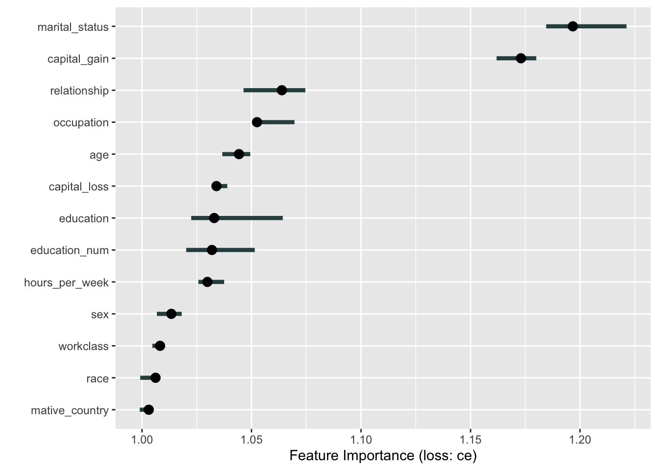
- Present the individual conditional expectations with the partial dependence plot overlaid across the range of values for the predictor X.
# Since I forgot to specify which predictor X... let's use education_num as an example!
# Why is this example harder to read and understand?
ice_with <- FeatureEffect$new(iml_model, feature = 'education_num',
                         method = 'pdp+ice', grid.size = 16)
ice_with$plot()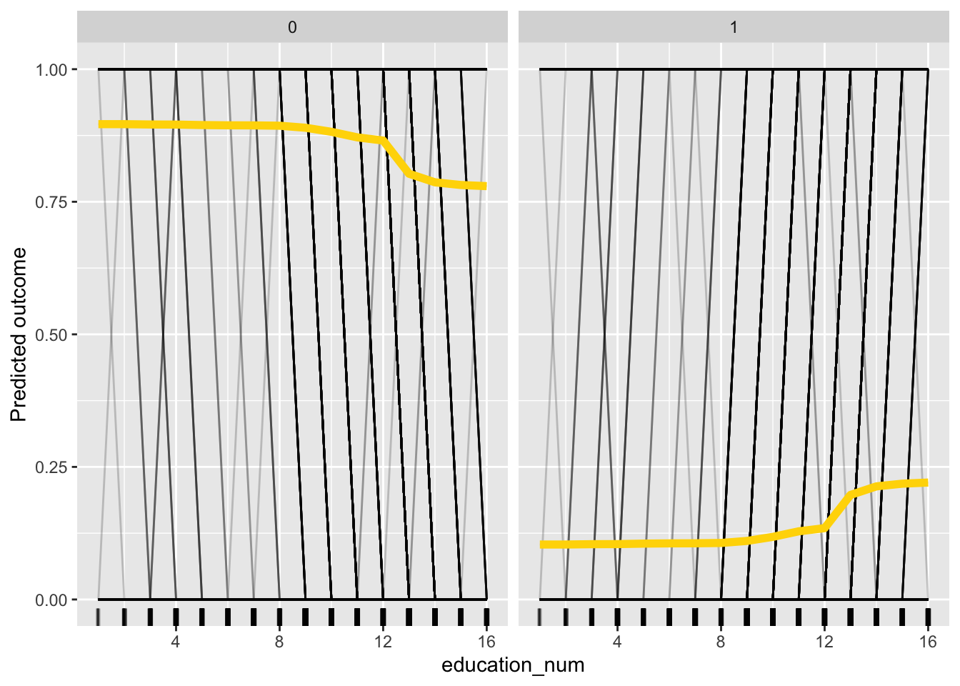
- Estimate a global surrogate with the logit model and a decision tree model. Present the regression table and the decision tree output. Which model is a better surrogate?
# since we want the outputs, we might consider estimating these global surrogate models
# outside the `iml` framework.

##Estimating first model
surr_logit <- glm(predicted_outcome~.,
              family = binomial,
              data = test_data %>%
                dplyr::select(-outcome)
              )
summary(surr_logit)
##
## Call:
## glm(formula = predicted_outcome ~ ., family = binomial, data = test_data %>%
## dplyr::select(-outcome))
##
## Coefficients: (2 not defined because of singularities)
## Estimate Std. Error z value Pr(>|z|)
## (Intercept) -3.448e+01 1.017e+03 -0.034 0.972951
## age 3.715e-02 9.279e-03 4.004 6.24e-05
## workclass Federal-gov 2.936e+00 8.060e-01 3.643 0.000270
## workclass Local-gov 2.045e+00 7.455e-01 2.743 0.006096
## workclass Never-worked -1.322e+01 1.100e+04 -0.001 0.999041
## workclass Private 1.858e+00 6.664e-01 2.788 0.005311
## workclass Self-emp-inc 3.131e+00 7.639e-01 4.099 4.15e-05
## workclass Self-emp-not-inc 6.349e-01 7.388e-01 0.859 0.390098
## workclass State-gov 1.239e+00 8.064e-01 1.537 0.124342
## workclass Without-pay -1.623e-01 1.126e+04 0.000 0.999988
## education 11th 1.505e+01 1.017e+03 0.015 0.988189
## education 12th 1.379e+01 1.017e+03 0.014 0.989180
## education 1st-4th 3.159e-01 2.459e+03 0.000 0.999898
## education 5th-6th 9.152e-01 1.965e+03 0.000 0.999628
## education 7th-8th -1.039e+00 1.457e+03 -0.001 0.999431
## education 9th 6.152e-01 1.674e+03 0.000 0.999707
## education Assoc-acdm 1.719e+01 1.017e+03 0.017 0.986512
## education Assoc-voc 1.617e+01 1.017e+03 0.016 0.987308
## education Bachelors 2.186e+01 1.017e+03 0.021 0.982851
## education Doctorate 2.529e+01 1.017e+03 0.025 0.980158
## education HS-grad 1.448e+01 1.017e+03 0.014 0.988639
## education Masters 2.254e+01 1.017e+03 0.022 0.982313
## education Preschool 3.914e+00 3.641e+03 0.001 0.999142
## education Prof-school 2.470e+01 1.017e+03 0.024 0.980618
## education Some-college 1.561e+01 1.017e+03 0.015 0.987755
## education_num NA NA NA NA
## marital_status Married-AF-spouse -8.682e+00 6.721e+03 -0.001 0.998969
## marital_status Married-civ-spouse 6.946e+00 1.694e+00 4.100 4.12e-05
## marital_status Married-spouse-absent -1.837e+00 1.623e+00 -1.132 0.257685
## marital_status Never-married -1.768e+00 7.611e-01 -2.323 0.020161
## marital_status Separated -8.255e+00 5.889e+00 -1.402 0.160966
## marital_status Widowed -1.055e+00 1.602e+00 -0.659 0.510179
## occupation Adm-clerical -2.360e+00 5.592e-01 -4.220 2.44e-05
## occupation Armed-Forces -1.483e+01 8.942e+03 -0.002 0.998677
## occupation Craft-repair -1.119e+00 4.623e-01 -2.421 0.015467
## occupation Exec-managerial 1.193e+00 4.280e-01 2.786 0.005330
## occupation Farming-fishing -4.289e+00 8.906e-01 -4.816 1.46e-06
## occupation Handlers-cleaners -2.374e+00 1.069e+00 -2.221 0.026337
## occupation Machine-op-inspct -1.351e+00 7.891e-01 -1.712 0.086859
## occupation Other-service -5.038e+00 1.186e+00 -4.249 2.15e-05
## occupation Priv-house-serv -2.286e+01 2.290e+03 -0.010 0.992038
## occupation Prof-specialty 3.436e-01 4.868e-01 0.706 0.480251
## occupation Protective-serv -1.030e+00 6.736e-01 -1.530 0.126130
## occupation Sales -2.670e-01 4.582e-01 -0.583 0.559998
## occupation Tech-support -5.814e-01 6.393e-01 -0.910 0.363071
## occupation Transport-moving NA NA NA NA
## relationship Not-in-family -5.343e-01 1.604e+00 -0.333 0.739064
## relationship Other-relative -2.328e+00 1.483e+00 -1.570 0.116388
## relationship Own-child -3.714e+00 1.653e+00 -2.247 0.024661
## relationship Unmarried -6.963e-01 1.913e+00 -0.364 0.715818
## relationship Wife 2.923e+00 7.894e-01 3.703 0.000213
## race Asian-Pac-Islander -6.236e-01 1.593e+00 -0.391 0.695540
## race Black -2.735e-02 1.307e+00 -0.021 0.983305
## race Other -1.608e+00 2.276e+00 -0.707 0.479695
## race White 3.101e-01 1.229e+00 0.252 0.800818
## sex Male 2.059e+00 6.975e-01 2.952 0.003159
## capital_gain 5.711e-04 4.008e-05 14.247 < 2e-16
## capital_loss 1.487e-03 1.664e-04 8.937 < 2e-16
## hours_per_week 4.307e-02 8.842e-03 4.871 1.11e-06
## mative_country Cambodia -1.103e+01 1.095e+04 -0.001 0.999196
## mative_country Canada -2.235e-01 1.810e+00 -0.123 0.901725
## mative_country China -9.666e-01 1.940e+00 -0.498 0.618275
## mative_country Columbia 5.032e-01 3.564e+03 0.000 0.999887
## mative_country Cuba 1.140e+00 1.496e+00 0.762 0.446053
## mative_country Dominican-Republic -5.931e+01 2.032e+04 -0.003 0.997671
## mative_country Ecuador -1.245e+01 1.092e+04 -0.001 0.999090
## mative_country El-Salvador -1.276e-01 2.745e+00 -0.046 0.962926
## mative_country England 7.459e-01 2.087e+00 0.357 0.720868
## mative_country France 6.973e-01 4.659e+00 0.150 0.881046
## mative_country Germany 1.991e+00 1.702e+00 1.170 0.242171
## mative_country Greece -6.502e-01 5.823e+00 -0.112 0.911083
## mative_country Guatemala -1.175e+01 3.609e+03 -0.003 0.997403
## mative_country Haiti -1.387e+01 4.245e+03 -0.003 0.997392
## mative_country Honduras -4.287e+00 1.119e+04 0.000 0.999694
## mative_country Hong -1.837e+00 2.078e+00 -0.884 0.376577
## mative_country Hungary -1.169e+01 8.090e+03 -0.001 0.998847
## mative_country India 2.100e-01 1.732e+00 0.121 0.903467
## mative_country Iran -1.018e+00 7.850e+00 -0.130 0.896776
## mative_country Ireland 4.022e+00 2.883e+00 1.395 0.162899
## mative_country Italy 1.622e+00 1.688e+00 0.961 0.336789
## mative_country Jamaica 9.704e-01 2.465e+00 0.394 0.693868
## mative_country Japan 3.218e+00 9.020e+00 0.357 0.721270
## mative_country Laos -1.195e+01 1.022e+04 -0.001 0.999067
## mative_country Mexico 4.801e-01 1.702e+00 0.282 0.777892
## mative_country Nicaragua 1.156e+00 5.642e+00 0.205 0.837708
## mative_country Outlying-US(Guam-USVI-etc) -1.317e+01 8.989e+03 -0.001 0.998831
## mative_country Peru -1.086e+01 8.565e+03 -0.001 0.998988
## mative_country Philippines 1.874e+00 1.681e+00 1.115 0.264926
## mative_country Poland -1.311e+00 2.024e+00 -0.648 0.517059
## mative_country Portugal 1.801e+00 1.227e+04 0.000 0.999883
## mative_country Puerto-Rico -4.973e-01 2.263e+00 -0.220 0.826091
## mative_country Scotland -1.445e+01 5.417e+03 -0.003 0.997871
## mative_country South 8.270e-01 1.803e+00 0.459 0.646432
## mative_country Taiwan 2.988e+00 2.011e+00 1.486 0.137382
## mative_country Thailand 2.136e+01 1.773e+04 0.001 0.999039
## mative_country Trinadad&Tobago -1.086e+01 1.042e+04 -0.001 0.999168
## mative_country United-States 9.242e-01 1.039e+00 0.890 0.373676
## mative_country Vietnam -4.604e+00 1.084e+02 -0.042 0.966120
## mative_country Yugoslavia -5.448e-01 1.773e+04 0.000 0.999975
##
## (Intercept)
## age ***
## workclass Federal-gov ***
## workclass Local-gov **
## workclass Never-worked
## workclass Private **
## workclass Self-emp-inc ***
## workclass Self-emp-not-inc
## workclass State-gov
## workclass Without-pay
## education 11th
## education 12th
## education 1st-4th
## education 5th-6th
## education 7th-8th
## education 9th
## education Assoc-acdm
## education Assoc-voc
## education Bachelors
## education Doctorate
## education HS-grad
## education Masters
## education Preschool
## education Prof-school
## education Some-college
## education_num
## marital_status Married-AF-spouse
## marital_status Married-civ-spouse ***
## marital_status Married-spouse-absent
## marital_status Never-married *
## marital_status Separated
## marital_status Widowed
## occupation Adm-clerical ***
## occupation Armed-Forces
## occupation Craft-repair *
## occupation Exec-managerial **
## occupation Farming-fishing ***
## occupation Handlers-cleaners *
## occupation Machine-op-inspct .
## occupation Other-service ***
## occupation Priv-house-serv
## occupation Prof-specialty
## occupation Protective-serv
## occupation Sales
## occupation Tech-support
## occupation Transport-moving
## relationship Not-in-family
## relationship Other-relative
## relationship Own-child *
## relationship Unmarried
## relationship Wife ***
## race Asian-Pac-Islander
## race Black
## race Other
## race White
## sex Male **
## capital_gain ***
## capital_loss ***
## hours_per_week ***
## mative_country Cambodia
## mative_country Canada
## mative_country China
## mative_country Columbia
## mative_country Cuba
## mative_country Dominican-Republic
## mative_country Ecuador
## mative_country El-Salvador
## mative_country England
## mative_country France
## mative_country Germany
## mative_country Greece
## mative_country Guatemala
## mative_country Haiti
## mative_country Honduras
## mative_country Hong
## mative_country Hungary
## mative_country India
## mative_country Iran
## mative_country Ireland
## mative_country Italy
## mative_country Jamaica
## mative_country Japan
## mative_country Laos
## mative_country Mexico
## mative_country Nicaragua
## mative_country Outlying-US(Guam-USVI-etc)
## mative_country Peru
## mative_country Philippines
## mative_country Poland
## mative_country Portugal
## mative_country Puerto-Rico
## mative_country Scotland
## mative_country South
## mative_country Taiwan
## mative_country Thailand
## mative_country Trinadad&Tobago
## mative_country United-States
## mative_country Vietnam
## mative_country Yugoslavia
## ---
## Signif. codes: 0 '***' 0.001 '**' 0.01 '*' 0.05 '.' 0.1 ' ' 1
##
## (Dispersion parameter for binomial family taken to be 1)
##
## Null deviance: 5636.15 on 6511 degrees of freedom
## Residual deviance: 783.95 on 6415 degrees of freedom
## AIC: 977.95
##
## Number of Fisher Scoring iterations: 19## Estimating second model
surr_rpart <- rpart(predicted_outcome~.,
data = test_data %>%
dplyr::select(-outcome)
)
rpart.plot::rpart.plot(surr_rpart)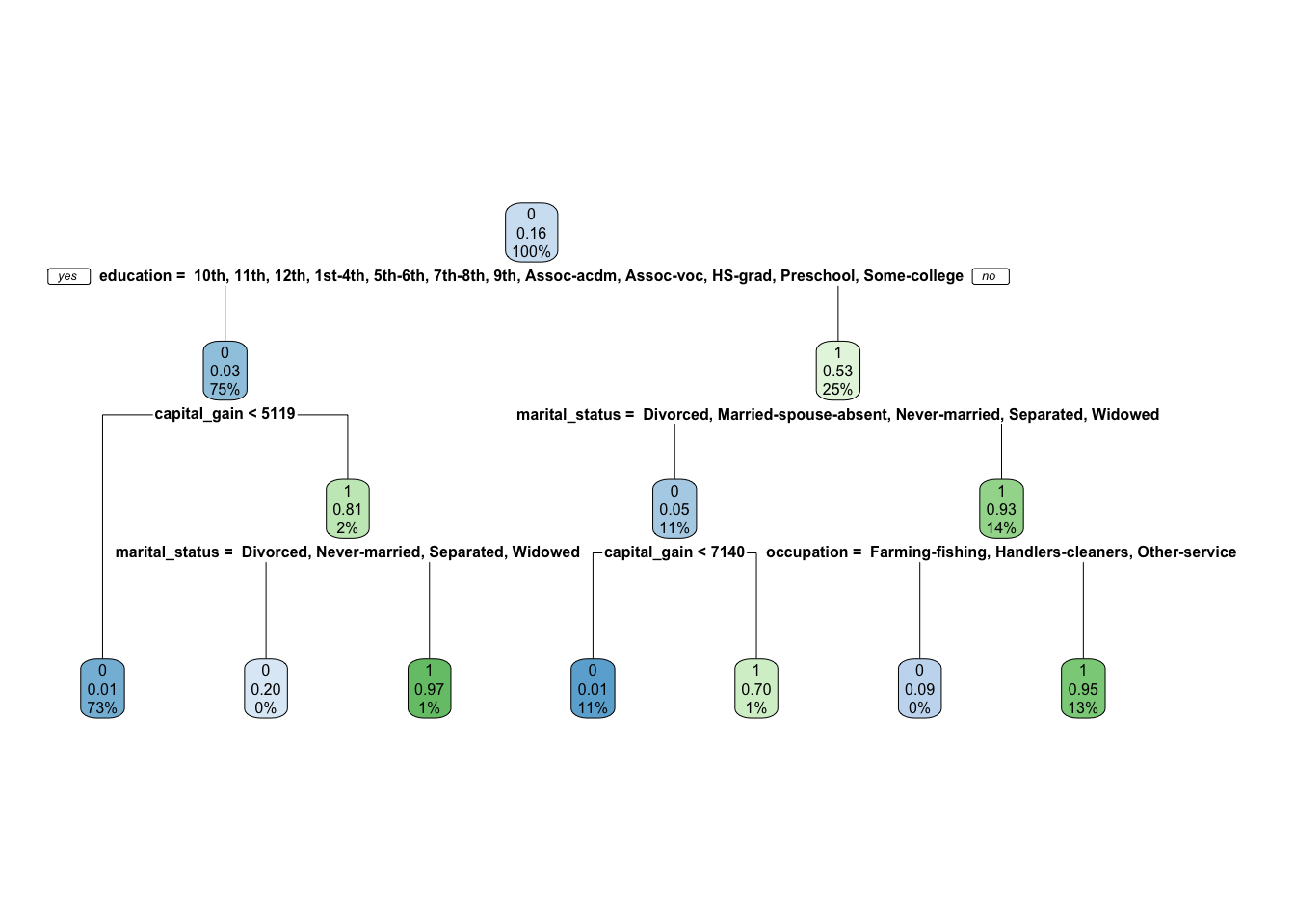
## Comparing
test_data <- test_data %>%
  mutate(predicted_logit = case_when(
    predict(surr_logit, ., type = 'response') < .5 ~  0,
    predict(surr_logit, ., type = 'response') >= .5 ~ 1
  ),
  predicted_rpart = case_when(
    predict(surr_rpart, ., type = 'class') == 0 ~ 0,
    predict(surr_rpart, ., type = 'class') == 1  ~ 1
  ),
  predicted_outcome = as.numeric(predicted_outcome)-1
  )


# Very similar performance! Both .98 accuracy
caret::confusionMatrix(as.factor(test_data$predicted_logit),
                       as.factor(test_data$predicted_outcome))
## Confusion Matrix and Statistics
##
## Reference
## Prediction 0 1
## 0 5448 76
## 1 49 939
##
## Accuracy : 0.9808
## 95% CI : (0.9772, 0.984)
## No Information Rate : 0.8441
## P-Value [Acc > NIR] : < 2e-16
##
## Kappa : 0.9263
##
## Mcnemar's Test P-Value : 0.02004
##
## Sensitivity : 0.9911
## Specificity : 0.9251
## Pos Pred Value : 0.9862
## Neg Pred Value : 0.9504
## Prevalence : 0.8441
## Detection Rate : 0.8366
## Detection Prevalence : 0.8483
## Balanced Accuracy : 0.9581
##
## 'Positive' Class : 0
## caret::confusionMatrix(as.factor(test_data$predicted_rpart),
as.factor(test_data$predicted_outcome))## Confusion Matrix and Statistics
##
## Reference
## Prediction 0 1
## 0 5440 64
## 1 57 951
##
## Accuracy : 0.9814
## 95% CI : (0.9778, 0.9846)
## No Information Rate : 0.8441
## P-Value [Acc > NIR] : <2e-16
##
## Kappa : 0.9292
##
## Mcnemar's Test P-Value : 0.5854
##
## Sensitivity : 0.9896
## Specificity : 0.9369
## Pos Pred Value : 0.9884
## Neg Pred Value : 0.9435
## Prevalence : 0.8441
## Detection Rate : 0.8354
## Detection Prevalence : 0.8452
## Balanced Accuracy : 0.9633
##
## 'Positive' Class : 0
##