Week 11 Optional Exercises (SOLUTIONS)
PPOL 6803
04/01/2026
Feel free to try the exercises below at your leisure. Solutions will be posted later in the week!
Text-as-Data
- Create a regular expression to find words that start with a vowel.
Test your findings on this vector
test <- c('apple', 'banana', 'kiwi', 'eggplant')
test <- c('apple', 'banana', 'kiwi', 'eggplant')

stringr::str_detect(test,
                    pattern = '^(a|e|i|o|u)')
## [1] TRUE FALSE FALSE TRUE- Scrape data from the body of the Wikipedia
page here. Using the
nrcsentiment library, summarize the proportion of non-stop words in each category. Compare your findings with a second Wikipedia page here.
get_sent_table <- function(url){
  raw <- read_html(url) %>%
    html_nodes('#bodyContent') %>%
    html_text2()

  raw <- data.frame(id = 1,
                    text = raw)

  output <- raw %>%
    unnest_tokens(output = 'word', input = 'text') %>%
    dplyr::anti_join(stop_words) %>%
    dplyr::mutate(ident = row_number()) %>%
    dplyr::mutate(unique_num = dplyr::n_distinct(ident)) %>%
    dplyr::inner_join(get_sentiments('nrc')) %>%
    dplyr::group_by(sentiment, unique_num) %>%
    dplyr::summarize(n = n()) %>%
    dplyr::ungroup() %>%
    dplyr::mutate(proportion = n/unique_num) %>%
    arrange(desc(proportion))
  return(output)
}

get_sent_table('https://en.wikipedia.org/wiki/R_(programming_language)')
## # A tibble: 10 × 4
## sentiment unique_num n proportion
## <chr> <int> <int> <dbl>
## 1 positive 5478 265 0.0484
## 2 trust 5478 143 0.0261
## 3 negative 5478 92 0.0168
## 4 anticipation 5478 79 0.0144
## 5 sadness 5478 65 0.0119
## 6 joy 5478 64 0.0117
## 7 fear 5478 18 0.00329
## 8 surprise 5478 17 0.00310
## 9 anger 5478 16 0.00292
## 10 disgust 5478 10 0.00183get_sent_table('https://en.wikipedia.org/wiki/Stata')## # A tibble: 10 × 4
## sentiment unique_num n proportion
## <chr> <int> <int> <dbl>
## 1 positive 3450 166 0.0481
## 2 negative 3450 100 0.0290
## 3 trust 3450 89 0.0258
## 4 anticipation 3450 71 0.0206
## 5 sadness 3450 58 0.0168
## 6 joy 3450 50 0.0145
## 7 fear 3450 23 0.00667
## 8 surprise 3450 22 0.00638
## 9 disgust 3450 15 0.00435
## 10 anger 3450 10 0.00290- Using the twitter data from the lab assignment (with the stop words
and other url link language excluded), produce a word cloud of the word
stems used in the tweets (use
SnowballC::wordStem()).
tweets <- read.csv("https://github.com/apodkul/ppol670_01/raw/main/Data/Climate_tweets.csv")

stop_words_2 <- data.frame(word =
                             c('https', 't.co'),
                           lexicon = 'custom')

tweets %>%
  mutate(tweet_id = 1:nrow(tweets)) %>%
  dplyr::select(tweet_id, text) %>%
  unnest_tokens(output = 'word', input = 'text') %>%
  anti_join(rbind(stop_words, stop_words_2)) %>%
  dplyr::filter(stringr::str_detect(word, pattern = '^[^0-9]*$')) %>%
  dplyr::mutate(word = SnowballC::wordStem(word)) %>%
  dplyr::count(word, sort = T) %>%
  filter(n > 150) %>%
  ggplot(aes(label = word, size = n)) +
  geom_text_wordcloud()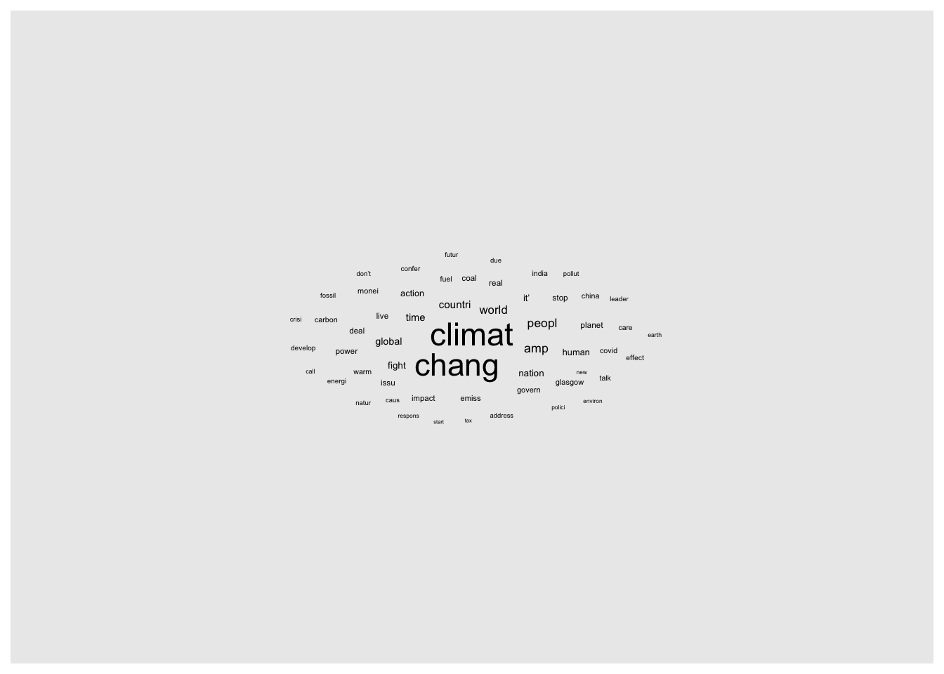
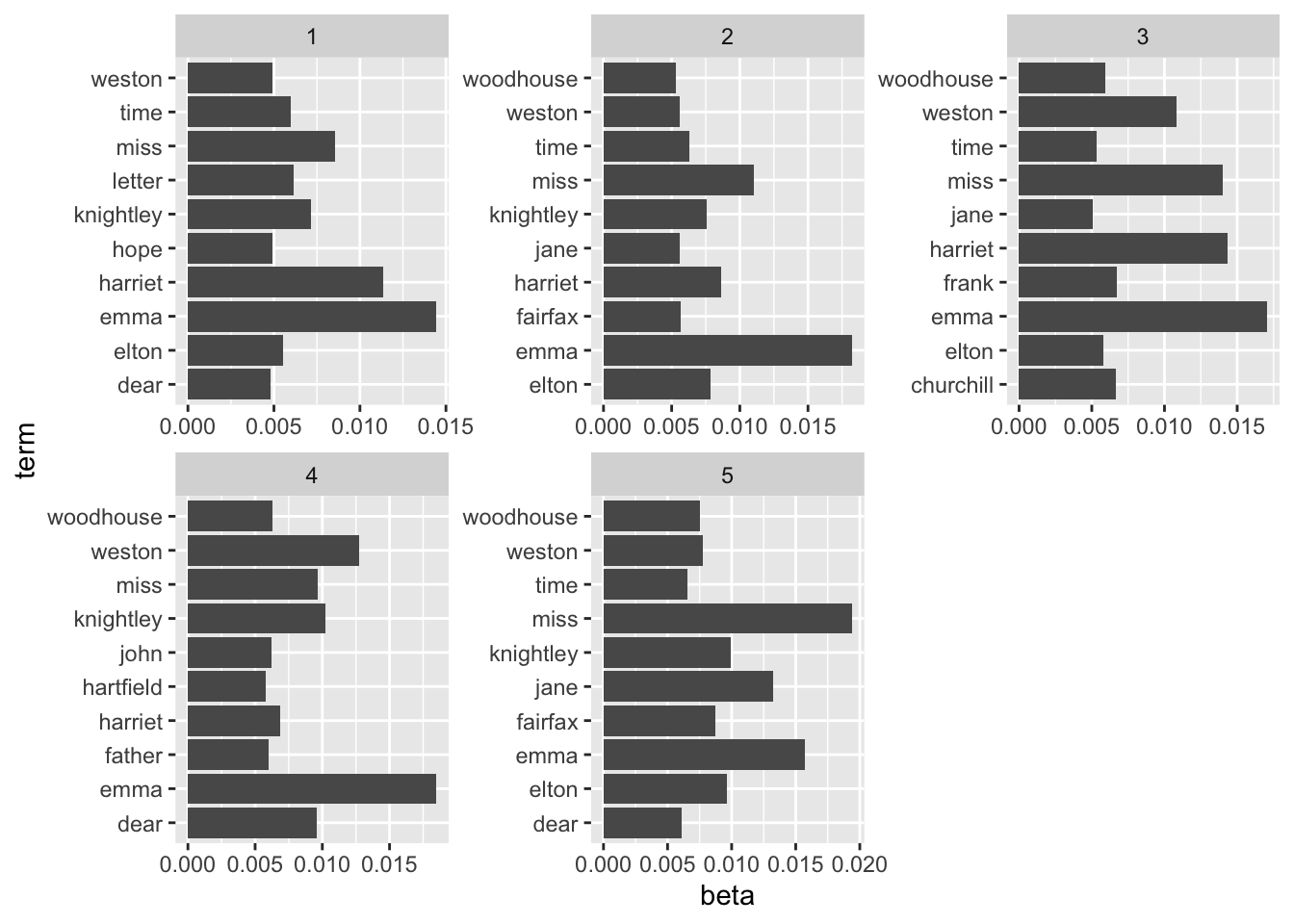
- Estimate a topic model for Jane Austen’s Emma (which can be
accessed in the
janeaustenrpackage). Estimate the model with 5 topics (treating chapters as documents). What are the top 10 words for each topic?
library(janeaustenr)
data("emma")

## Preprocess to convert to terms, documents
emma <- data.frame(line = 1:length(emma),
                   text = emma)
emma$chapter_break <- stringr::str_detect(emma$text,
                                      pattern = 'CHAPTER') # Note chapters are nested in Volumes, ignoring
emma$chapter <- cumsum(emma$chapter_break)

emma <- emma %>%
  dplyr::filter(chapter != 0 & text != '') %>%
  dplyr::select(chapter, text) %>%
  unnest_tokens(output = 'word', input = 'text') %>%
  dplyr::anti_join(stop_words) %>%
  dplyr::group_by(chapter) %>%
  dplyr::count(word)

#Convert to document term matrix
emma_dtm <- emma %>%
  cast_dtm(chapter, word, n)

#Run LDA model
emma_model <- LDA(x = emma_dtm, k = 5)

#Identify top 10 words for each (using beta terms)
tidy(emma_model, matrix = 'beta') %>%
  group_by(topic) %>%
  slice_max(beta, n = 10) %>%
  ggplot() +
  geom_bar(aes(x = beta, y = term), stat = 'identity') +
  facet_wrap(~topic, scales = 'free')